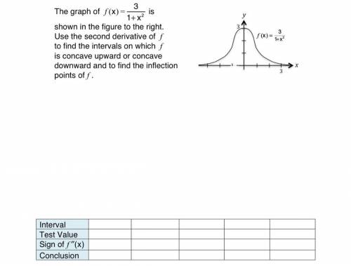
Concave Up Interval: 
Concave Down Interval: 
General Formulas and Concepts:
Calculus
Derivative of a Constant is 0.
Basic Power Rule:
f(x) = cxⁿf’(x) = c·nxⁿ⁻¹
Quotient Rule: ![\frac{d}{dx} [\frac{f(x)}{g(x)} ]=\frac{g(x)f'(x)-g'(x)f(x)}{g^2(x)}](/tpl/images/0929/2566/a2a0e.png)
Chain Rule: ![\frac{d}{dx}[f(g(x))] =f'(g(x)) \cdot g'(x)](/tpl/images/0929/2566/44454.png)
Second Derivative Test:
Possible Points of Inflection (P.P.I) - Tells us the possible x-values where the graph f(x) may change concavity. Occurs when f"(x) = 0 or undefinedPoints of Inflection (P.I) - Actual x-values when the graph f(x) changes concavityNumber Line Test - Helps us determine whether a P.P.I is a P.I
Step-by-step explanation:
Step 1: Define

Step 2: Find 2nd Derivative
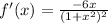
1st Derivative [Quotient/Chain/Basic]:
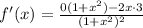
Simplify 1st Derivative:
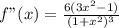
2nd Derivative [Quotient/Chain/Basic]:
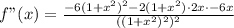
Simplify 2nd Derivative:
Step 3: Find P.P.I
Set f"(x) equal to zero:

Case 1: f" is 0
Solve Numerator:
Divide 6:

Add 1:

Divide 3:

Square root:

Simplify:

Rewrite:

Case 2: f" is undefined
Solve Denominator:

Cube root:

Subtract 1:

We don't go into imaginary numbers when dealing with the 2nd Derivative Test, so our P.P.I is (x ≈ ±0.57735).
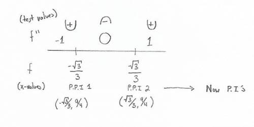
Step 4: Number Line Test
See Attachment.
We plug in the test points into the 2nd Derivative and see if the P.P.I is a P.I.
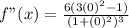
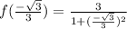
x = -1
Substitute:
Exponents:
Multiply:
Subtract/Add:

Exponents:

Multiply:

Simplify:

This means that the graph f(x) is concave up before  .
.
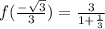
x = 0
Substitute:
Exponents:
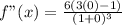
Multiply:
Subtract/Add:

Exponents:

Multiply:

Divide:

This means that the graph f(x) is concave down between and .
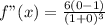
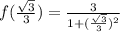
x = 1
Substitute:
Exponents:
Multiply:
Subtract/Add:
Exponents:
Multiply:
Simplify:
This means that the graph f(x) is concave up after  .
.
Step 5: Identify
Since f"(x) changes concavity from positive to negative at and changes from negative to positive at , then we know that the P.P.I's are actually P.I's.
Let's find what actual point on f(x) when the concavity changes.
Substitute in P.I into f(x):
Evaluate Exponents:
Add:

Divide:

Substitute in P.I into f(x):
Evaluate Exponents:

Add:

Divide:

Step 6: Define Intervals
We know that before f(x) reaches , the graph is concave up. We used the 2nd Derivative Test to confirm this.
We know that after f(x) passes , the graph is concave up. We used the 2nd Derivative Test to confirm this.
Concave Up Interval:
We know that after f(x) passes , the graph is concave up until . We used the 2nd Derivative Test to confirm this.
Concave Down Interval: